Inicio este post parafraseando Duncan Watts, autor do livro “Tudo é óbvio*”, onde explora “como o senso comum nos engana” e oferece uma nova maneira de pensar. Dr. Watts foi pesquisador-chefe do Yahoo! Research e foi um dos pioneiros nos estudos das dinâmicas sociais através da facilidade e revolução da internet e das redes. Trouxe questionamentos e ofereceu respostas fundamentadas em dados que, segundo ele, são indispensáveis a “empresários, políticos, cientistas e todos nós.”
Meu primeiro contato com este livro fora logo após o seu lançamento — estava escancarado na entrada de uma das minhas livrarias-café favoritas de Porto Alegre. Sua tão exposta obviedade passou batida, exceto por aquele incômodo asterisco vermelho, já sinalizando a promessa registrada em sua capa.
O exemplar impresso, repousado em minha estante, está marcado por anotações e destaques de uma leitura realizada quando ainda trabalhava com inovação e desenvolvimento de novas tecnologias, em meados de 2012. Éramos um time relativamente pequeno e discutíamos projetos que, anos mais tarde, viriam a impactar o dia a dia de milhões de pessoas. Dito isto, tornam-se óbvias as razões que me levaram a grifar o seguinte trecho:
“(..) Um número pequeno de pessoas sentadas em salas de conferência está usando sua intuição do senso comum para prever, gerenciar ou manipular o comportamento de milhares ou milhões de pessoas distantes e diversas cujas motivações e circunstâncias são muito diferentes das suas.”
D. Watts, 2011. “Tudo é Óbvio* Desde que você saiba a resposta.” P. 35.
Hoje, uma década mais tarde, refaço a leitura e retomo tais anotações — agora com o privilégio de poder validá-las. Minhas atividades e perspectivas mudaram, assim como o próprio mundo mudou. A rede social predominante à época e que inspirou muitas das análises do Dr. Watts, o Twitter, segue sendo extremamente ativa. Agora, porém, disputa a largura de banda com tantas outras redes e se inunda em grandes lagos de informação (mais conhecidos como data lakes). As salas de conferência também foram inundadas por dados e hoje, pode-se dizer, são minimamente híbridas: combinações entre universos e metaversos.
É neste contexto que a intuição do senso comum cedeu lugar à intuição baseada em dados — isto é, aos modelos de machine learning. O objetivo, porém, em nada mudou: seguimos buscando modelos para “prever, gerenciar ou manipular o comportamento” e, dada sua sofisticação, presumimos que sua qualidade tenha melhorado.
Estariam os algoritmos, portanto, isentos do viés causado pelo senso comum?
Minha intenção ao repercorrer os capítulos desta obra — cujas reflexões compartilharei por aqui — é justamente questionar o impacto na ciência de dados causado pelo viés do senso comum, assim como do “problema do enquadramento”, “problema micro-macro”, “viés retrospectivo”, dentre tantos outros apontados pelo autor.
Are you interested in data science, and are you aware of the situation of COVID-19 in Brazil? In this post, I will explore the concept of data acquisition and demonstrate how to use a simple web scraping technique to obtain official data on the progress of the disease. It is worth saying that, with some adaptation in the code, the strategy used here can be easily extended to data from other countries or even to other applications. So put on your mask, wash your hands, and start reading it right now!
I must start this text offering the most sincere sentiments to all victims of COVID-19. It is in their memory that we must seek motivation for the development of science without forgetting that if it exists, it is because there is a humanity that sustains it. Concerning data science, it is through it that we can minimize fake news and somehow contribute to a more informed, sensible, and thoughtful society.
I started this data analysis project when I realized, a few weeks ago, that there was little stratified information on the number of cases of COVID-19 in Brazil on official bases, such as that of the World Health Organization (WHO – World Health Organization) or the panel maintained by John Hopkins University. As stratified, in fact, we understand the set of data that can be observed in different layers. That is, for a country of continental dimensions, such as Brazil, knowing the total number of cases in the country is only informative. For such information to be functional, it must be stratified by regions, states, or cities.
To provide both an overview of the problem and direct the development of the analysis, I have set out below some objectives for this study that I hope the reader will appropriate them too:
Acquire an overview of the KDD process and understand where the data acquisition places on it.
Explore data acquisition techniques so that similar problems could easily employ them.
Obtain, from official databases, the number of cases and deaths by COVID-19 in Brazil, stratified by state.
In the following sections, we will explore each of these items to build the necessary concepts and implement them in a Python development environment. Ready?
KDD – Knowledge Discovering in Databases
Knowledge discovery in databases is the process by which someone seeks for comprehensive, valid, and relevant patterns from databases. It is an interactive and iterative process, which comprises many of the techniques and methods that are known today as data science.
Before exploring the main stages of the KDD process, however, it is worth differentiating three key terms: data, information, and knowledge. Each step of KDD is concerned with processing each of these terms, illustrated in the diagram of Fig. 1 from the problem we are working on.
Figure 1. From data to knowledge: information processing in KDD.
In short, data are all chains of symbols, structured or not, related to some phenomenon or event. Data, by itself, has no meaning. See: the 4.08 million number is just a cardinal. It becomes scary only after we assign it the sense that this is the number of confirmed cases of COVID-19. In other words, we have information only when we assign meaning to data.
It is from the manipulation of information that we acquire knowledge, which is closely related to what we call “cognitive processes” — perception, contextualization, and learning — and, therefore, intelligence.
Once these three concepts are understood, we can now proceed to the three fundamental phases of the KDD process. These are nothing more than sets of tasks respectively dedicated to obtaining and exploring data, information, and knowledge, as illustrated in Fig. 2, below:
Figure 2. The KDD process and its phases of (i) data acquisition, (ii) information processing, and (iii) knowledge extraction.
The KDD process consists of steps, which in turn are compound of tasks. Data mining tasks, for example, are part of the information processing step. In contrast, those tasks related to data visualization, analytics, and decision making are part of the last step, which aims for knowledge extraction.
In this article, we will focus only on the data acquisition task, fundamental to any KDD project. In general, there is no predefined method for obtaining data. Medium and long term projects usually demand a data model, as well as a robust architecture for its collection and storage. Short-term projects, in turn, mostly require immediately available and accessible sources.
With these fundamental concepts in mind, we are ready to move towards our purpose: the acquisition of official data on the number of COVID-19 cases in Brazil.
Defining a data acquisition strategy
As we have seen, a data acquisition strategy will only make sense if built from the perspective of a complete KDD process. That is, before we start collecting data out there, we need to have a clear purpose definition. What is the problem that we are trying to solve or elucidate?
The CRISP-DM reference model, shown in Fig.3, can be used as a compass when going through a KDD process. Do you remember that we previously defined KDD as an interactive and iterative process?
Well, the interaction means mutual or shared action between two or more agents. It can refer either to people holding data and information or to the stages. The short arrows, in both directions between the first steps of Fig. 3, represent the necessary interaction in the process. I dare say it is the biggest challenge for newcomers to the world of KDD or data science: there is an initial illusion that these steps follow a continuous flow, which results in a feeling of doing something wrong. Quite the contrary, by understanding the business, we make it possible to understand the data, which gathers us new insights about the business, and so on.
Iteration, in turn, is associated with the repetition of the same process. The larger arrows, in Fig.3, form a circle that symbolizes this repetition. It starts in the first step and returns, after development, to it again. A KDD project will never be stagnant.
Figure 3. Phases of the KDD process according to the CRISP-DM reference model. (Adapted from Wikimedia Commons.)
The highlighted boxes, in Fig. 3, represent the steps related to the data acquisition process. According to CRISP-DM, the first step — understanding the business — is fundamental to the success of the entire project and comprises (i) the definition of the business objectives; (ii) the assessment of the current situation, including inventories and risk analyzes, as well as what data and information are already available; (iii) the determination of the objectives in applying data mining, and also the definition of what the success criteria will be; and (iv) the elaboration of a project plan.
The second step — understanding the data — comprises (i) the first data samples and (ii) its detailed description; (iii) the initial exploration of the data; and (iv) an assessment of the quality of that data. Remember that these two initial steps take place interactively and, ideally, involving domain and business specialists.
The third step begins with the validation of the project plan by the sponsor and is characterized by the preparation of the data. In general, the efforts required in this phase become more expensive and, therefore, their changes should be milder. The main tasks of this step include the selection and cleaning of data, the construction and adaptation of the format, and the merging of data. All of these tasks are commonly referred to as data pre-processing.
Your data acquisition strategy will start being defined as soon as you have the first interactions between understanding the business (or the problem) and following the available data. For that, I consider essentially two possible scenarios:
There is control over the data source: you can somehow manage and control the sources that generate the data (sensors, meters, people, databases, etc.). Take, for example, the activity of a head nurse: he can supervise, audit, establish protocols, and record all patient data in his ward. It is important to note that the control is over the origin or registration of the data, and not over the event to which the data is related. This scenario usually happens in projects of high complexity or duration, where a data model is established, and there are means to ensure its consistency and integrity.
There is no control over the data source: this is the most common situation in projects of short duration or of occasional interest, as well as in projects, analyzes, or perennial studies that use or demand data from sources other than their own. Whatever the initiative, the data acquisition strategy must be more reliable, given that any change beyond its control can increase the costs of its analysis or even render the project unfeasible. Our own study illustrates this scenario: how to obtain the stratified number of COVID-19 cases in Brazil if we have no control over the production and dissemination of these data?
Expect to find the first scenario in corporations and institutions, or when leading longitudinal research or manufacturing processes. Otherwise, you will likely have to deal with the second one. In this case, your strategy may consist of subscriptions, data assignment agreements, or even techniques that search and compile such data from the Internet, once they are properly licensed. Web scraping is one of these techniques, as we will see next.
Data acquisition via web scraping: obtaining data with the official panel of the Brazilian Ministry of Health
With the objective established — the stratified number of COVID-19 cases in Brazil — my first action was to look for possible sources. I consulted the Brazilian Ministry of Health web portal in mid-April, 2020. At the time, I had not found consolidated and easily accessible information, so I increased the granularity of possible sources: state and municipal health departments. The challenge, in this case, was the heterogeneity in the way they presented the data. When consulting a public health worker, she informed me that the data were consolidated in the national bulletins and that specific demands should be requested institutionally. My first strategy, then, was to devise a way to automatically collect such bulletins (in PDF format) and start extracting the desired data — part of the result is available in this GitHub repository.
At the beginning of May 2020, though, I had an unpleasant surprise: the tables I had used to extract the data (for those who are curious, the PDFplumber library is an excellent tool) were replaced by figures, in the news bulletins, which made my extraction method unfeasible.
I made a point of going through the above paragraphs in detail for a simple reason: to demonstrate, once again, the interactive process inherent to the data acquisition step in KDD. Besides, I wanted to highlight the risks and uncertainties when we took on a project where we have no control over the data source. In these situations, it is always good to have alternatives, establish partnerships or agreements, and seek to build your own dataset.
While I was looking for a new strategy, the Brazilian Ministry of Health started making the data available into a single CSV file — days later changing the format to XLSX and changing the file name every day. In the following paragraphs, I will detail how I adapted my process and code for this new situation.
By the way, the automatic retrieval of data and information from pages and content made available on the Internet is called web scraping. This technique can be implemented effortlessly through Python libraries, as shown in Fig. 4.
Figure 4. The steps of a simplified web scraping process using the Google Chrome inspection tool and the Python language.
We finally come to the practical — and perhaps the most anticipated — part of this text. Following the steps defined in Fig. 4, we start by (1) visiting the Coronavirus panel and (2) identifying that our interest is in the data made available by clicking on the “Arquivo CSV” button in the upper right corner of the page. When we activate the Google Chrome page inspection tool (3), we find the code corresponding to the item on the HTML page, as shown in Fig. 5. Remembering that the inspection tool is activated by the Inspect menu, when we right-click over any element of the page, or by the shortcut ctrl+shift+I.
Figure 5. Coronavirus portal from Brazilian Ministry of Health seen through the Google Chrome Inspection tool.
The next step (4) is to access this data from our code in Python, which can go through Jupyter notebooks, scripts, or through an IDE. In any case, the idea is to emulate the access to the desired portal and the interaction with the web page by using the Selenium library.
In the lines below, I start creating a virtual environment to access the portal URL within the Google Chrome emulator:
# Initial statements
from pyvirtualdisplay import Display
from selenium import webdriver

# Parameters definition
url = 'https://covid.saude.gov.br'
## A linha abaixo pode ser suprimida em alguns ambientes:
chromeDriverPath = '~/anaconda3/envs/analytics3/'

# Starts the virtual environment:
display = Display(visible=0, size=(800,600))
display.start()

# Opens the Chrome emulator in the desired URL:
driver = webdriver.Chrome()

# Reads and gets the page content encoded in UTF-8:
driver.get(url)
page = driver.page_source.encode('utf-8')
Once we read the page, we proceed to step (5) of Fig. 4, where we iterate the process until we guarantee that the data is in our desired form. To do so, we can start by checking the size of the loaded page (e.g., if it is null, it means something went wrong) and its first lines:
# What is the length of the loaded page?
print(len(page))

# What is the data type?
print(type(page))

# What is the content of the first positions of the byte stream?
print(page[:2000])
Most of the time, the next step would be to explore HTML content using tools known as parsers — the BeautifulSoup library is an excellent parser for Python. In our case, considering that the data we are interested are not on the web page but result from an action on this page, we will continue using only the Selenium methods to emulate the click on the button, automatically downloading the desired file for the default system folder:
## Path obtained from inspection in Chrome:
xpathElement = '/html/body/app-root/ion-app/ion-router-outlet/app-home/ion-content/div[1]/div[2]/ion-button'

## Element corresponding to the "Arquivo CSV" button:
dataDownloader = driver.find_element_by_xpath(xpathElement)

## Download the file to the default system folder:
dataDownloader.click()
The next step is to verify if the file was downloaded correctly. Since its name is not standardized, we then list the recent files through the glob library:
import os
import glob

## Getting the last XLSX file name:
list_of_files = glob.glob('/home/tbnsilveira/Downloads/*.xlsx')
latest_file = max(list_of_files, key=os.path.getctime)
print(latest_file)
From this point on, the web scraping task is completed, at the same time that we enter the data preparation phase (if necessary, review Fig. 3).
Let’s consider that we are interested in the number of cases per state, concerning its population, as well as in the lethality rates (number of deaths to the number of cases) and mortality (number of deaths to the number of people). The lines of code below perform the pre-processing tasks needed to offer the desired information.
## Reading the data
covidData = pd.read_excel(latest_file)
covidData.head(3)

## Getting the last registered date:
lastDay = covidData.data.max()

## Selecting the dataframe with only the last day
## and whose data is consolidated by state
covidLastDay = covidData[(covidData.data == lastDay) &
                         (covidData.estado.isna() == False) &
                         (covidData.municipio.isna() == True) &
                         (covidData.populacaoTCU2019.isna() == False)]

## Selecting only the columns of interest:
covidLastDay = covidLastDay[['regiao','estado','data','populacaoTCU2019','casosAcumulado','obitosAcumulado']]
The pre-processing step is completed by generating some additional features, from the pre-existing data:
## Copying the dataframe before handling it:
normalCovid = covidLastDay.copy()

## Contamination rate (% of cases by the population of each state)
normalCovid['contamRate'] = (normalCovid['casosAcumulado'] / normalCovid['populacaoTCU2019']) * 100
## Fatality rate (% of deaths by the number of cases)
normalCovid['lethality_pct'] = (normalCovid['obitosAcumulado'] / normalCovid['casosAcumulado']) * 100
## Mortality rate (% of deaths by the population in each state)
normalCovid['deathRate'] = (normalCovid['obitosAcumulado'] / normalCovid['populacaoTCU2019']) * 100
From this point, we can search in the pre-processed database:
normalCovid.query("obitosAcumulado > 1000")
Here we end the data acquisition phase. If we follow the CRISP-DM methodology, the next steps could be either the construction of models, analyzes, or visualizations. To illustrate a possible conclusion of this KDD process, Fig. 6 presents a Four-Quadrant graph correlating the percentage of cases versus the lethality rate in the different states of Brazil (the code to generate it is available on GitHub).
Figure 6. Relationship between the number of COVID-19 cases and lethality, by states in Brazil, according to data released by the Ministry of Health on 05/22/2020.
The graphic above is the result of the entire process we covered so far: the data was obtained via web scraping, the information was generated from the manipulation of that data, and the knowledge was acquired by structuring the information. Amazonas (AM) is the state population with the highest number of infections per inhabitant, as well as with the highest lethality rate. São Paulo (SP) is the state with the highest cumulative number of deaths, but with a relatively low number of infections considering its entire population.
Final considerations
In this article, I tried to offer an overview of the KDD process and how to implement data acquisition using a web scraping technique, especially in the case of small projects or analyzes.
You may have wondered if it wouldn’t be much easier just to visit the web portal and simply download the data available there. Yes, it would! However, a data science project expect data acquisition as automatic as possible, giving space to move forward with predictive analyzes whose models require daily or constant updating. Also, understanding complex topics and gaining confidence about our technique becomes much more effective — and perhaps amusing — with relatively more straightforward problems.
Finally, I must remind you to always act ethically in the acquisition and manipulation of data. Automating the collection of data in the public domain, at no cost to its administration, is characterized as a completely legal activity. However, if you are in doubt as to when the use of such algorithms is allowed or not, do not hesitate to consult experts or even the data owners.
If you have followed the article so far, I would love to hear your opinion. In addition to the poll below, feel free to leave a comment or write to me with any questions, criticisms or suggestions.
Lean Six Sigma is a continual improvement methodology broadly applied in the production and services industries. In this post series, we will run through it by applying such tools in this blog-writing process.
A year ago, I decided to restart writing a blog. I was excited about sharing my research ideas, some data analysis code, and some daily findings or even ramblings. I should mention that I had yet created an editorial calendar with well-meaning and already started posts.
But as you can suppose by reading this now, I wrote nothing more and a full year has passed before I show up again. I would be lying if saying my willingness to write has changed. Indeed it may have even increased. So why didn’t I write?
A trivial answer would be to blame the lack of time — in fact, this was one of the busiest years of my last decades. However, this alone does not explain the whole story. In this way, I decided to apply the Lean Six Sigma (L6S) methodology to my blog writing activity. After all, having started my Green Belt certification, alongside several other demands, could be part of my naive justification of my (non-)writing.
Lean Six Sigma methodology
In short, L6S is a continual improvement methodology that seeks to make processes leaner and more efficient by reducing its variability and waste. Its history is related to the production management programs developed by Motorola and Toyota, among other companies, throughout the 1980s and 1990s. These, in turn, are based on the statistical process control, whose development and application began in the 1920s. Currently, the L6S methodology is adopted by numerous companies and has an international standardization (ISO 13053, first released in 2011).
The most common L6S methodology is known as DMAIC, standing for its five compounding phases, as follow:
DMAIC methodology and its compounding phases (Source: Wikimedia Commons.)
Define: in this phase, an overview of the process is drawn by observing its main problems, as well as establishing the goals and catching a glimpse of the ways out. This phase outcome is a project chart describing the problem, the project scope, and the expected benefits.
Measure: once the problem has been defined, this phase is intended to collect the largest amount of meaningful information regarding it. Such data become a baseline for validating the process improvement.
Analyze: this phase seeks to analyze the data collected during the last one (and which will continue to be collected). The primary outcome must be an in-depth analysis of the problems root causes. For this task, there are many statistical tests available in the L6S toolbox.
Improve: based on the previous phases, here we propose solutions for the identified problems supported by the evidence found. The main outcome is the new process map (as it should be) with a set of actions to be implemented.
Control: in this final phase, a control plan is developed both to measure the effectiveness of the actions undertaken, as well as ensuring they will be kept accordingly.
My certification is still in progress — which, in addition to the theoretical training, involves leading a continual improvement project with proven financial results to the company I work for. Applying such a robust methodology in a blog writing process should be seen as an exercise since it is a personal endeavor that does not carry any financial KPI as most of the corporate processes.
Processes can be continually improved
Before we dive into the first phase of the L6S methodology, it is affordable to discuss how activities can be understood as a process. First of all, a process is a recurrent activity that has inputs; operations or functions to process the inputs; and outputs, these last resulting from the processing of the inputs.
A process on its most basic form: the input x is processed by the function f(x), resulting in the output y.
I usually distinguish a process from a system by considering the latter as composed of many processes. In the diagram below, we can find a more complex version of our basic process. In this case, the single input x is replaced by the set X of m inputs. We may also have more than an output, now represented by the set Y of n outputs. In turn, our system is represented by the set F of c functions or operations.
A process on its most beautiful complex form: the set of inputs X is processed by the set of functions F, resulting in the set of outputs Y.
Although one may successfully apply the L6S methodology without using the notation above for the system and its processes, understanding such formalization can be very useful for statistical analysis and automation. In any case, what we want is to improve our system in the way that the functions in F will perform as best as possible. In other words, our ideal system should output the best Y values for a given set X of inputs.
By using the L6S tools we become able to avoid failures and to optimize our processes to a minimum wasting rate. However, since any process in our universe obeys to the thermodynamics laws (remember them here), we must always expect some wastes.
In this context, the sigma value of a given process tells us how many failures (or wastes) are expected on every million occurrences (measured in DPMO – defects per million opportunities). As a reference, in a six sigma process the DPMO value is only 3.4, i.e., in such processes, only 3.4 failures are allowed for every 1 million occurrences.
The blog-writing process
Fortunately, many events can be described as processes, as is the case with scientific writing and blog writing. In both cases, the inputs can be the reasons why someone should write, or so his/her objectives. The operations of functions are the writing process itself. Obviously, the output is the text in its final version.
From my perspective, the most serious flaw is easy to identify: the text is simply not published, i.e., its output is not delivered.
I hope to have the opportunity to detail how fun and surprising it can be to apply such a robust methodology to a relatively simple and personal problem. The message I want to leave, for now, is that a method such as L6S makes us rethink what the real aims of the process are; what tools do we have to evaluate them; and how the results are being achieved. In short, it makes us able to answer these kinds of questions:
What did I want by creating this blog?
Why did the writing not occur?
What can be done to make this process efficient, i.e., to deliver what is expected?
If we look closely, we can see how much these questions are related to strategic planning. Hence the relevance of applying L6S for the most diverse applications. If, in your case, there is a well-defined strategic plan, the L6S will undoubtedly help you to improve it. Otherwise, this will be one of the first needs identified by the methodology and, best of all, by using L6S you won’t have to create a strategic plan from scratch.
Did you get interested? In the next post of this series, I will explore which L6S tools will help me answer the first question. Follow the blog to be notified. Until then!
If you have ever heard Python and Fourier nouns, chances are you’ll find this post useful: here I will explore a simple way to implement the Short-Time Fourier Transform in Python in order to run a frequency analysis for a given signal. Let’s get to work!
A few weeks ago I was invited to join a Kaggle’s competition with my colleagues from my research group. The idea has sounded very interesting to me since it is about seismic data, i.e. time series, which is somehow related to the signal category I was used to working with — for the curious ones, I have applied wavelets for drowsiness detection from brain signals. By the way, wavelet analysis has become famous when Stéphane Mallat applied it to seismic and geological data.
But before we start dealing with wavelets (which I do intend to get back to them in the near future), the main idea here is to get acquainted with periodic signals. I mean, a time series representing some cyclic events that repeat from time to time. And that, therefore, can be often designated as a pattern.
You may find patterns represented in the most different forms, but one, in particular, is the circle: the day and the night time, the seasons of the year, the electricity generated in hydroelectric, all of them are related to a circular source (or at least an approximated one, since the Earth is an oblate spheroid which orbits the Sun in an elliptical path).
From a mathematical perspective, any cyclic pattern can be somehow represented by the trigonometric sine and cosine functions, as demonstrated by the French mathematician and physicist Joseph Fourier, who in the early nineteenth century has established what is known today as Fourier Series and Fourier Transform.
The sine and cosine functions are the projections of a circular movement over a vertical and horizontal axis, respectively.
I will assume you are already familiar with trigonometric signals and their relation with frequency. In any case, what is important to notice is that a periodic or cyclic signal will repeat itself by a given amount of time, known as period (T). The frequency (f), in turn, consists of the number of repetitions per second and is measured in hertz (Hz), in homage to the German physicist Heinrich Hertz.
In the next sections, we will explore these concepts in a very practical way (I’m also assuming you are used to Python). We will first figure out how to generate and visualize some periodic waves (or signals), moving then to a Short-Time Fourier Transform implementation. For last, we will see an example of how to apply such analysis for a non-trigonometric function but rhythmic one, as the brain signals.
1. Generating periodic signals
In data science — and here I’m considering all the disciplines related to it, such as pattern recognition, signal processing, machine learning and so on — it is always useful to have a deep understanding of how our data (a.k.a. signals) behave when inserted into an analysis or classification tool. The problem is that at first we usually know little about our data — which in the real world can be complex and noisy — and in fact, looking for analytical tools is an attempt to understand them.
In these cases, the best alternative is to explore the analysis tool with simple and well-known data. Paraphrasing the Nobel laureate Richard Feynman — who left in his blackboard the following quote, after his death in 1988: “What I can not create, I do not understand” –, we will first generate our own periodic signals.
A time series usually results from a sampling process effort. When this signal is generated, as is the case here, we must also establish the time where the signal supposedly occurs. The function below emulates the sampling process and has as input the initial and the final time samples. In other words, it returns the x-axis basis where our signal will be placed.
[code language="python"]
import numpy as np

def timeSeries(fs, ti, tf):
    '''Returns a time series based on:
        fs = the sampling rate, in hertz (e.g. 1e3 for 1kHz);
        ti = the starting time (e.g. second 0);
        tf = the final time (e.g. second 1).'''
    T = 1./fs
    timeSeries = np.arange(ti,tf,T)
    return timeSeries
[/code]
Let’s remember that a sinusoidal signal is generated by the function: , where f is the frequency, in hertz, of the signal y(t), and t is the time series generated by the code above. This equation is then transcripted to Python:
[code language="python"]
def genSignal(freq, amp, timeSeries):
    '''Returns the time series for a sinusoidal signal, where:
        freq = frequency in Hertz (integer);
        amp = signal amplitude (float);
        timeSeries = the linear time series (array).'''
    signal = amp*np.sin(freq*2*np.pi*timeSeries)
    return signal
[/code]
Almost as important as generating the signal is to provide a means of visualizing it. Using the Matplotlib library, the following function can be adapted to view any time series:
[code language="python"]
import matplotlib.pyplot as plt

def plotSignal(signal, timeSeries, figsize=(6,3)):
    '''signal = numpy.array or Pandas.Series;
        timeSeries = the linear time series x-axis;
        figsize = the plot size, set as (6,3) by default.'''
    fig, axes = plt.subplots(1,1, figsize=figsize)
    plt.plot(timeSeries, signal)
    #Adjust the ylim to go 10% above and below from the signal amplitudes
    axes.set_ylim(signal.min()+signal.min()*0.1, signal.max()+signal.max()*0.1)
    axes.grid(True)
    axes.set_ylabel('Signal amplitude')
    axes.set_xlabel('Time (s)')
    return
[/code]
It also sounds practical to code a wrapper function to create and visualize a sinusoidal function getting frequency and amplitude as input parameters:
[code language="python"] def sineWave(freq, amp, timeSeries):
    '''Generates and plots a sine wave using genSignal() and plotSignal().
        freq = frequency in Hertz (int);
        amp = signal amplitude (float);
        timeSeries = a linear time series accordingly to the sample rate.'''
    signal = genSignal(freq, amp, timeSeries)
    plotSignal(signal, timeSeries)
    return signal [/code]
Finally, we will now execute these functions together in order to obtain some sinusoidal waves:
[code language='python']
import numpy as np
import matplotlib.pyplot as plt
%matplotlib inline

## Sampling time for 0s to 10s, 1kHz:
time = timeSeries(1e3,0,10)

## Generating a sine wave of 1Hz and amplitude of 2:
sign1 = sineWave(1, 2, time)

## Generating a sine wave of 0.1Hz and amplitude of 1:
sign01 = sineWave(0.1, 1, time)
[/code]
Which then give us the following result:
It may look quite simpler, but it is important to have a signal which we know exactly how it was created — we hold its model, i.e. its formula. Observe in the first chart above that a frequency of 0.1Hz means the signal will repeat itself every 10 seconds. In the second chart, we duplicate the amplitude of the signal which now repeats its pattern every second.
Putting together the functions we have defined with the numpy.concatenate method, as shown below, we can generate more complex waveforms:
[code language='python']
# Generating two segmented time series:
time1 = timeSeries(fsLANL,0,1)
time2 = timeSeries(fsLANL,1,2)
# Concatenating them in order to plot:
time = np.concatenate((time1, time2), axis=None)

# Generating the signals for each time series:
signal1 = genSignal(20,50,time1)
# Here we add up two frequencies:
signal2 = genSignal(113,28,time2) + genSignal(70,53,time2) + genSignal(0.25,30,time2)
# Concatenating both signals
signal = np.concatenate((signal1,signal2), axis=None)

# Plotting the resulting signal:
plotSignal('[0.25, 20, 70, 113]', signal, time, figsize=(12,6))
[/code]
From our first charts, it becomes clear that when we are dealing with low and single frequencies we can still identify cyclic patterns only through visual inspection in the time domain signals (e.g. counting the tops during a second). However, for more complex waves (see the interval between 1s and 2s in the chart above) it becomes clear that a tool is needed to identify any cyclic pattern.
2. The Short-Time Fourier Transform
A complete understanding of time series representation in the frequency domain requires a deepening of linear algebra and calculus for expanding a signal in a series of functions.
Such an approach, though, will not be taken here: those who already understand this mathematical abstraction would find a practical code for implementing a frequency analysis in Python. In the same way, those who are facing periodic signals for the first time may start deepening their theoretical understanding from these simple examples.
Before we start coding, I will provide a brief definition (please don’t get scared with the symbols… If you want, you may just page down to skip this block): Fourier has proved that it is possible to expand a great number of functions into pure harmonic functions series (i.e. a sum of sines and cosines). By the way, from the Euler’s formula we know we can represent harmonic functions as a complex exponential:
.
Now consider that we can expand a given signal y(t) into a Fourier Series:
, where are the Fourier coefficients obtained by the Fourier transform of the signal; and is the harmonic base function that represents the frequency .
What is important to have in mind is that each coefficient — what our computer will be calculating for us — is associated with a harmonic base function, which in turn relates this coefficient to a specific frequency. Then, if we know the value of each coefficient, we could know the intensity of each frequency component present in the signal y(t).
Another important aspect one should consider is that these base functions have infinite duration and therefore are not suitable for representing signals with discontinuities or of which the location in time or space is also desired (i.e. when we seek to know in which period of the signal a given frequency or rhythm happens the most).
The Short-Time Fourier Transform (STFT) is a way to overcome this. Its strategy consists of multiplying each basis function of the transform by a window function, w(t). This last thus being limited to a given period of time, i.e. having non-null values just for a limited interval.
Considering the function space in the Fourier transform can be defined by trigonometric functions in its complex form, for the STFT we create a new basis defined both by frequency () and position ():
, .
The shape and length of w(t) must be chosen accordingly to the analysis interest. The shape depends on the function used to generate it and determines its capability of frequency resolution. On the other hand, the length (N) defines the window interval and therefore its temporal resolution.
Many window functions can be used and tried out (an overview of their main features and differences can be found here). For our purpose — or when in doubt about which one to pick — the Hann window can be a satisfying choice:
Let us now return to our Python code. Once we have understood the basic principles the STFT relies on, we can make use of the signal module from SciPy library to implement an spectrogram — which consist of plotting the squared magnitude of the STFT coefficients.
So, with the code below we will compute the STFT for our first signal (page up and seek for the sign1). Also, we must consider that the SciPy implementation will always set the frequency axis accordingly to half of the sampling frequency, the reason why I set the plt.ylim() command.
Okay, I do agree with you that this result is far short of what I expected. The good news is that (almost) everything is a matter of adjustment. To make things easier, let’s write the following function:
[code language='python']
def calcSTFT(inputSignal, samplingFreq, window='hann', nperseg=256, figsize=(9,5), cmap='magma', ylim_max=None, output=False):
    '''Calculates the STFT for a time series:
        inputSignal: numpy array for the signal (it also works for Pandas.Series);
        samplingFreq: the sampling frequency;
        window : str or tuple or array_like, optional
            Desired window to use. If `window` is a string or tuple, it is
            passed to `get_window` to generate the window values, which are
            DFT-even by default. See `get_window` for a list of windows and
            required parameters. If `window` is array_like it will be used
            directly as the window and its length must be nperseg. Defaults
            to a Hann window.
        nperseg : int, optional
            Length of each segment. Defaults to 256.
        figsize: the plot size, set as (6,3) by default;
        cmap: the color map, set as the divergence Red-Yellow-Green by default;
        ylim_max: the max frequency to be shown. By default it's the half sampling frequency;
        output: 'False', as default. If 'True', returns the STFT values.

        Outputs (if TRUE):
            f: the frequency values
            t: the time values
            Zxx: the STFT values"'''
    ##Calculating STFT
    f, t, Zxx = signal.stft(inputSignal, samplingFreq, window=window, nperseg=nperseg)
    ##Plotting STFT
    fig = plt.figure(figsize=figsize)
    ### Different methods can be chosen for normalization: PowerNorm; LogNorm; SymLogNorm.
    ### Reference: https://matplotlib.org/tutorials/colors/colormapnorms.html
    spec = plt.pcolormesh(t, f, np.abs(Zxx),
                          norm=colors.PowerNorm(gamma=1./8.),
                          cmap=plt.get_cmap(cmap))
    cbar = plt.colorbar(spec)
    ##Plot adjustments
    plt.title('STFT Spectrogram')
    ax = fig.axes[0]
    ax.grid(True)
    ax.set_title('STFT Magnitude')
    if ylim_max:
        ax.set_ylim(0,ylim_max)
    ax.set_ylabel('Frequency [Hz]')
    ax.set_xlabel('Time [sec]')
    fig.show
    if output:
        return f,t,Zxx
    else:
        return
[/code]
To test it, we will create a new signal whose values are easy to understand and manipulate, a 100Hz sine wave with amplitude 1000. Since we will keep it lasting 10s, with the same sampling rate of 1kHz, we can use the array time defined before.
[code language='python']
fs = 1e3  #The sampling frequency
test = genSignal(100,1000,time)  #Generating the signal

calcSTFT(test, fs)  #Calling our function in its simplest form!
[/code]
It looks so much better now!!
The purpose to start with a simple signal is that it allows us to check whether there is a gross error in our code or not. Fortunately, it’s not the case! The plot frequency range goes up to 500Hz, half the sampling frequency, as expected. Also, we can precisely see the 100Hz component, which values are normalized (you will find the details on the normalization strategy here).
Going further, we can specify other parameters to our STFT. To create the charts below I set different values for the nperseg parameter, which correspond to the window function size. For the left image, nperseg = 64, while for the right one nperseg = 2048. Note how a larger window results in a much more accurate frequency resolution. And vice versa.
There is no specific rule to determine the number of samples per segment. However, it’s useful to consider 1/4 of the sampling rate. E.g. for a 1kHz sampling rate, the nperseg parameter is set by default to 256. This tradeoff can become clearer if we analyze our complex signal, which we generated with components from 0.25 to 123Hz:
In the plot above all the known frequency components of the signal become evident, although there is lower time resolution. For some applications, 250ms are insignificant. For others, it can be limiting. I must anticipate to you that there is no analytical tool that may offer accuracy both in time and frequency, as demonstrated by the Heisenberg’s principle — but this will be subject for a next post.
3. Brain signal analysis
To exemplify how the STFT analysis can be useful for “real life” situations, we will now apply the functions we built on a brain signal segment obtained from electroencephalography (EEG). If you want to try it on your own, the data is available here.
Since the signal was previously processed on Matlab, we will first have to convert the data structure to a Python dictionary using the loadmat method. Knowing that the signal was labeled as sD_W, we can move on to loading it:
[code language='python']
import scipy.io
mat = scipy.io.loadmat('brainSignal.mat')

brain_raw = mat['sD_W']
## Checking the shape of the variable:
brain_raw.shape

## Adequating the signal to an np.array
brain = brain_raw.T[0]

## Plotting the brain signal:
plt.plot(brain)

## Calculating its STFT
calcSTFT(brain, 200, nperseg=2**8, figsize=(9,4), ylim_max=100, cmap='inferno')
[/code]
Time domain.Time-frequency domain.
Unlike when dealing with sinusoidal signals, now we can’t deduce the rhythms (i.e. frequency components) present in the EEG signal only by looking to its time domain plot. We could even say that something is happening after 20s, but we could not give any detail.
On the other hand, the spectrogram above shows us that after the event around 20s, a well established low-frequency rhythm appears from 20s to 36s and then again from 44s to 56s. As with any data science activity, the interpretation is always context-dependent. In this case, this EEG signal is from a subject submitted to polysomnography. The identified frequency range corresponds to the alpha rhythm, indicating that the patient is probably awake and relaxed, but with closed eyes. For last, the dark region around 50Hz corresponds to a pass-band filter applied during the signal acquisition in order to filter the 50Hz interference from AC power supply.
4. Conclusions
The goal of this post was not only to show how to implement STFT in Python, but also to bring a brief introduction to the theory behind this powerful analytical tool — which supports the more intricate ideas of mathematics.
Also, by being able to understand the main parameters that should be observed in such analysis, and drawing on the example with brain signals, I hope the reader may tailor the code and apply such a tool to any cyclic signal he/she may find: from biomedical or seismic signals going even to stock market prices or the movement of stars.
Você tem interesse em data science e está sensibilizado com a situação da COVID-19 no Brasil? Neste post, irei explorar o conceito de data acquisition e demonstrar como utilizar uma técnica simples de web scraping para obter dados oficiais sobre o avanço da doença. Vale dizer que, com alguma adaptação no código, a estratégia aqui empregada pode ser facilmente estendida a dados de outros países ou ainda a outras aplicações. Então ponha sua máscara, lave suas mãos e inicie a leitura agora mesmo!
Devo iniciar este texto, antes de tudo, oferecendo os mais sinceros sentimentos a todas as vítimas da COVID-19. De fato, é em memória destes que devemos buscar motivação para o desenvolvimento da ciência, em todas as suas áreas e expressões, sem esquecermos de que se ela existe é porque há uma humanidade que a sustenta. Em relação à ciência de dados, é através dela que podemos minimizar fake news e contribuir, de alguma forma, com uma sociedade mais informada, sensata e ponderada.
Iniciei este projeto de exploração de dados ao perceber, há algumas semanas atrás, que havia pouca informação estratificada sobre o número de casos da COVID-19 no Brasil em bases oficiais, tais como a da Organização Mundial da Saúde (WHO – World Health Organization) ou do painel mantido pela Universidade John Hopkins. Como estratificado, aliás, entende-se o conjunto de dados que pode ser observado em diferentes camadas. Ou seja, para um país de dimensões continentais, como o Brasil, saber o número total de casos no país é apenas informativo. Para que tal informação seja funcional, ela deve ser estratificada por regiões, estados, ou cidades.
De modo a proporcionar tanto uma visão geral do problema quanto direcionar o desenvolvimento da análise, estabeleci abaixo alguns objetivos para este estudo dos quais espero que o leitor também se aproprie:
Adquirir uma visão geral do processo de KDD e compreender onde a aquisição de dados está inserida.
Explorar técnicas de aquisição de dados de modo que possam ser facilmente empregadas em problemas e casos similares.
Obter, a partir de bases de dados oficiais, o número de casos e óbitos por COVID-19 no Brasil, estratificado por estado.
Nas seções a seguir, exploraremos cada um desses itens buscando construir os conceitos necessários e implementá-los de maneira prática em um ambiente de desenvolvimento em Python. Prontos?
KDD – Descobrindo conhecimento em bases de dados
A descoberta de conhecimento em bases de dados, mais conhecida por sua sigla KDD, do inglês Knowledge Discovery in Databases, é o processo pelo qual se busca padrões compreensíveis, válidos, e relevantes a partir de bases de dados. É um processo interativo e iterativo, que compreende muitas das técnicas e processos conhecidos atualmente como ciências de dados.
Antes de explorarmos as principais etapas do processo de KDD, porém, vale diferenciarmos três termos-chaves: dados, informações e conhecimento. Cada etapa do processo de KDD, aliás, ocupa-se de processar cada um desses termos, ilustrados no diagrama da Fig. 1 a partir da problemática em que estamos trabalhando.
Figura 1. Dos dados ao conhecimento: o processamento da informação no KDD.
Em resumo, dados são todas as cadeias de símbolos, estruturadas ou não, relacionadas a algum fenômeno ou evento. Um dado, por si, não traz significado algum. Veja: o número 4,08 milhões é apenas um cardinal inteiro. Ele se torna assustador somente após atribuirmos a ele o significado de que esta é a quantidade de casos confirmados da COVID-19. Ou seja, somente ao atribuirmos um significado a um dado é que passamos a ter uma informação.
É a partir da manipulação da informação que adquirimos conhecimento. Este, por sua vez, está íntima e etimologicamente ligado ao que chamamos de “processos cognitivos” — a percepção, a contextualização e o aprendizado — e, por conseguinte, à inteligência.
Uma vez compreendidos estes três conceitos, podemos agora avançar para as três etapas fundamentais do processo de KDD. Estas nada mais são do que conjuntos de tarefas respectivamente dedicadas à obtenção e exploração dos dados, informações e conhecimento, conforme ilustrado na Fig. 2, abaixo:
Figura 2. O processo de KDD e suas etapas de (i) aquisição dos dados, (ii) processamento das informações e (iii) extração do conhecimento.
O processo de KDD, portanto, é constituído de etapas e cada qual, de tarefas. As tarefas de data mining, por exemplo, fazem parte da etapa de processamento da informação, enquanto que as tarefas relacionadas à visualização de dados, analytics, e tomada de decisão constituem a última etapa, pela qual se extrai o conhecimento.
Neste artigo, vamos nos deter somente à tarefa de aquisição de dados (data acquisition), fundamental a todo e qualquer processo de KDD. De modo geral, não existe um método pré-definido e generalista para a obtenção dos dados. Em um projeto de médio e longo prazos, normalmente desenvolve-se um modelo de dados e uma arquitetura robusta para a sua coleta e armazenamento. Já em projetos de curto prazo, ou então em análises como esta, utilizam-se as fontes imediatamente disponíveis e acessíveis que mais estejam relacionadas ao problema.
Tendo estes conceitos fundamentais em mente, estamos prontos para seguir em direção ao nosso propósito: a aquisição de dados oficiais sobre o número de casos da COVID-19.
Definindo uma estratégia de aquisição de dados
Como vimos, uma estratégia de aquisição de dados só fará sentido se for construída a partir da perspectiva de um processo completo de KDD. Isto é, antes de sairmos coletando dados por aí, precisamos ter bem definido qual é o propósito disto tudo. Ou ainda, qual é o problema que estamos tentando resolver ou elucidar?
O modelo de referência CRISP-DM, representado na Fig.3, pode ser utilizado como uma bússula ao percorrermos um processo de KDD. Você se recorda que anteriormente definimos o KDD como um processo interativo e iterativo?
Pois bem, a interação pode ser definida como a ação mútua ou compartilhada entre dois ou mais agentes. Neste caso, a interação pode se referir tanto entre as pessoas detentoras de dados e informações, ou entre as etapas. As setas curtas, em ambos os sentidos entre os primeiros passos da Fig. 3, representam justamente a interação necessária no processo. Ouso dizer que tal interação é o maior desafio dos recém-chegados ao mundo do KDD ou data science: há uma ilusão inicial de que os passos devem ser seguidos em um fluxo contínuo, o que logo decorre em uma sensação de se estar fazendo algo errado. Muito pelo contrário, é a compreensão do negócio que possibilita a compreensão dos dados, que gera novos insights sobre o negócio e assim por diante.
A iteração, por sua vez, está associada à repetição do mesmo processo. As setas maiores, na Fig.3, formam um círculo que simboliza esta repetição. Inicia-se no primeiro passo e retorna-se, após o desenvolvimento, novamente a ele. Enquanto estiver ativo, um projeto de data science ou KDD nunca ficará estagnado.
Figura 3. Fases do processo de KDD de acordo com o modelo de referência CRISP-DM.(Adaptado de Wikimedia Commons.)
As caixas destacadas, na Fig. 3, representam os passos relacionados à aquisição de dados, sendo nelas que iremos nos deter a partir daqui, embora de modo um tanto simplificado.
De acordo com o CRISP-DM, o primeiro passo — a compreensão do negócio — é fundamental para o sucesso de todo o projeto e compreende (i) a definição dos objetivos do negócio; (ii) a avaliação da situação atual, incluindo inventários e análises de risco, bem como quais dados e informações já estão disponíveis; (iii) a determinação dos objetivos em se aplicar data mining, assim como a definição de quais serão os critérios de sucesso; e (iv) a elaboração de um plano de projeto.
O segundo passo — o entendimento dos dados — compreende (i) a coleta inicial dos dados e (ii) sua descrição detalhada; (iii) a exploração inicial dos dados; e (iv) uma avaliação da qualidade desses dados. Lembre-se de que estes dois passos iniciais ocorrem de maneira interativa e, idealmente, envolvendo especialistas de domínio e de negócio.
O terceiro passo inicia-se com a validação do plano de projeto pelo cliente ou pelo sponsor e caracteriza-se pela preparação dos dados. Em linhas gerais, os esforços necessários nesta fase tornam-se maiores e, portanto, suas alterações devem ser mais brandas. As principais tarefas desta etapa compreendem a seleção e limpeza dos dados, a construção e a adequação do formato, e a integração de dados (merging). Todas essas tarefas são normalmente referidas como pré-processamento dos dados.
Sua estratégia de aquisição de dados começará a ser definida tão logo você tenha as primeiras interações entre a compreensão do negócio (ou do problema) e o entendimento dos dados disponíveis. Para tanto, considero essencialmente dois cenários possíveis:
Há controle sobre a origem dos dados: você pode, de algum modo, gerenciar e controlar as fontes geradoras dos dados (sensores, medidores, pessoas, bancos de dados, etc.). Tome, como exemplo, a atividade de um enfermeiro-chefe: ele pode supervisionar, auditar, estabelecer protocolos e realizar o registro de todos os dados de pacientes em sua enfermaria. É importante salientar que o controle é sobre a origem ou registro dos dados, e não sobre o evento ao qual os dados estão relacionados. Este é geralmente o cenário de projetos de grande complexidade ou duração, onde se estabelece um modelo de dados e se estabelecem meios para garantir sua consistência e integridade.
Não há controle sobre a origem dos dados: esta é a situação mais comum em projetos de curta duração ou de interesse ocasional, assim como projetos, análises ou estudos perenes que utilizem ou demandem dados de outras fontes que não as próprias. Seja qual for a iniciativa, a estratégia de aquisição de dados deve ser ainda mais fortalecida, dado que qualquer alteração — que está além do seu controle — pode aumentar os custos de sua análise ou mesmo inviabilizar o projeto. Este cenário é ilustrado pelo nosso próprio estudo: como obter o número estratificado de casos da COVID-19, no Brasil, se não temos controle sobre a produção e divulgação destes dados?
Espere encontrar o cenário (1) ao atuar em ambientes corporativos e instituições, ou ao liderar pesquisas longitudinais ou então processos de fabricação. De outro modo, é bem provável que você tenha de lidar com o cenário (2). Neste caso, sua estratégia poderá compor-se de subscrições (assinatura de serviços), acordos de cessão de dados, ou ainda de técnicas que busquem e compilem tais dados a partir da Internet, desde que devidamente licenciados. A atividade de web scraping é uma destas técnicas, como veremos a seguir.
Aquisição de dados por web scraping: obtendo os dados via painel oficial do Ministério da Saúde
Uma vez estabelecido o objetivo — o número estratificado de casos da COVID-19 no Brasil — minha primeira ação foi buscar quais seriam as possíveis fontes. Consultei o portal do Ministério da Saúde em meados de Abril/2020. Na ocasião, não havia encontrado informações consolidadas e de fácil acesso, de modo que aumentei a granularidade das possíveis fontes: secretarias estaduais e municipais de saúde. O desafio, neste caso, foi a heterogeneidade no modo com que os dados eram apresentados (quando eram). Ao consultar uma servidora pública da área da saúde, fui informado de que os dados eram consolidados nos boletins, e que demandas específicas deveriam ser solicitadas institucionalmente. Minha primeira estratégia, então, foi elaborar um meio de automaticamente coletar tais boletins (em formato PDF) e começar a extrair deles os dados desejados — parte do resultado está disponível no repositório GitHub deste projeto.
No início de Maio/2020, porém, tive uma desagradável surpresa: as tabelas que até então eu utilizara para extrair os dados de meu interesse (para quem tiver curiosidade, a biblioteca PDFplumber é uma excelente ferramenta) foram substituídas por figuras, nos novos boletins, o que inviabilizou o meu método de extração.
Fiz questão de discorrer em detalhes os parágrafos acima por uma simples razão: demonstrar, mais uma vez, o processo interativo inerente à etapa de aquisição de dados, no KDD. Além disso, quis evidenciar os riscos e incertezas ao assumirmos um projeto onde não temos controle sobre a origem dos dados. Nessas situações, é sempre bom contar com alternativas, estabelecer parcerias ou convênios, e buscar construir sua própria base de dados.
Ao passo em que eu buscava uma nova estratégia, o Ministério da Saúde passou a disponibilizar os dados já compilados em um único arquivo CSV — dias depois alterando o formato para XLSX e variando o nome do arquivo a cada dia. Nos parágrafos a seguir, detalharei como adequei meu processo e meu código para esta nova situação.
A propósito, a obtenção automática de dados e informações a partir de páginas e conteúdos disponibilizados na Internet é denominada web scraping. Tal técnica pode ser implementada de maneira bastante simples, utilizando bibliotecas disponíveis em Python, conforme esquematizado na Fig. 4.
Figura 4. Etapas de um processo simplificado de web scraping utilizando a ferramenta de inspeção do Google Chrome e a linguagem Python.
Chegamos finalmente à parte prática — e talvez a mais esperada — deste texto. Seguindo as etapas definidas na Fig. 4, começamos por (1) visitar o Painel Coronavírus Brasil e (2) identificar que o nosso interesse está nos dados disponibilizados ao clicarmos no botão “Arquivo CSV”, no canto superior direito da página. Ao ativarmos a ferramenta de inspeção de páginas do Google Chrome (3), localizamos o código correspondente ao item na página HTML, conforme mostrado na Fig. 5. Lembrando que a ferramenta de inspeção é ativada pelo menu Inspecionar, ao clicarmos com o botão direito sobre algum elemento da página, ou pelo atalho ctrl+shift+I.
Figura 5. Portal Coronavírus Brasil visto através da ferramenta de inspeção do Google Chrome.
O passo seguinte (4) é acessar estes dados a partir de linhas de código em Python, o que pode ser feito através de cadernos do Jupyter, scripts, ou através de uma IDE. Em qualquer dos casos, a ideia é emular o acesso ao portal desejado e a interação com a página web, utilizando para isso a biblioteca Selenium.
No código abaixo, inicio criando um ambiente virtual para em seguida acessar o site de interesse com o emulador do Google Chrome:
# Declarações iniciais
from pyvirtualdisplay import Display
from selenium import webdriver

# Definição de parâmetros
url = 'https://covid.saude.gov.br'
## A linha abaixo pode ser suprimida em alguns ambientes:
chromeDriverPath = '~/anaconda3/envs/analytics3/'

# Inicializa o display (tela virtual):
display = Display(visible=0, size=(800,600))
display.start()

# Abre o emulador do Chrome para o site desejado:
driver = webdriver.Chrome()

# Lê o conteúdo da página, armazenando-o em UTF-8:
driver.get(url)
page = driver.page_source.encode('utf-8')
Uma vez realizada a leitura da página, seguimos para o passo (5) da Fig. 4, onde iteramos o processo até garantir a obtenção dos dados na forma desejada. Para tanto, podemos iniciar verificando o tamanho da página carregada (se for nulo, significa que algo deu errado) e suas primeiras linhas:
# Qual é o tamanho da página carregada?
print(len(page))

# Qual é o tipo de dados?
print(type(page))

# Qual é o conteúdo das primeiras posições do fluxo de bytes?
print(page[:2000])
Na maioria das vezes, o passo seguinte seria explorar o conteúdo HTML através de ferramentas conhecidas como parsers — a biblioteca BeautifulSoup cumpre muito bem esta função em Python. No nosso caso, considerando que os dados de interesse não estão na página web, mas sim resultam de uma ação nesta página, iremos seguir utilizando apenas os métodos do Selenium para emular o clique sobre o botão, automaticamente fazendo o download do arquivo desejado para a pasta padrão do sistema:
## Caminho obtido a partir da inspeção no Chrome:
xpathElement = '/html/body/app-root/ion-app/ion-router-outlet/app-home/ion-content/div[1]/div[2]/ion-button'

## Elemento correspondente ao botão "Arquivo CSV":
dataDownloader = driver.find_element_by_xpath(xpathElement)

## Download do arquivo para a pasta padrão do sistema:
dataDownloader.click()
O passo seguinte é verificarmos se o download do arquivo foi realizado corretamente. Dado que o nome do arquivo não é padronizado, a listagem é feita através da biblioteca glob:
import os
import glob

## Obtendo o nome do arquivo XLSX mais recente:
list_of_files = glob.glob('/home/tbnsilveira/Downloads/*.xlsx')
latest_file = max(list_of_files, key=os.path.getctime)
print(latest_file)
A partir deste ponto, podemos considerar finalizada a tarefa de web scraping, ao mesmo tempo em que adentramos na fase de preparação dos dados (se necessário, reveja a Fig. 3).
Vamos considerar que estamos interessados na quantidade de casos por estado, em relação à sua população, assim como nas taxas de letalidade (número de óbitos em relação ao número de casos) e de mortalidade (número de óbitos em relação à população). As linhas de código abaixo realizam o pré-processamento dos dados obtidos de modo a oferecer as informações desejadas.
## Leitura dos dados
covidData = pd.read_excel(latest_file)
covidData.head(3)

## Obtendo a última data registrada:
lastDay = covidData.data.max()

## Selecionando o dataframe apenas com os dados do último dia
## E cujos dados sejam consolidados por estado
covidLastDay = covidData[(covidData.data == lastDay) &
                         (covidData.estado.isna() == False) &
                         (covidData.municipio.isna() == True) &
                         (covidData.populacaoTCU2019.isna() == False)]

## Selecionando apenas as colunas de interesse:
covidLastDay = covidLastDay[['regiao','estado','data','populacaoTCU2019','casosAcumulado','obitosAcumulado']]
A etapa de pré-processamento é concluída ao gerarmos algumas features adicionais, a partir dos dados pré-existentes:
## Cópia do dataframe antes de manipulá-lo:
normalCovid = covidLastDay.copy()

## Taxa de contaminação (% de casos pela população de cada estado)
normalCovid['contamRate'] = (normalCovid['casosAcumulado'] / normalCovid['populacaoTCU2019']) * 100
## Taxa de letalidade (% de óbtiso pelo núm. casos)
normalCovid['lethality_pct'] = (normalCovid['obitosAcumulado'] / normalCovid['casosAcumulado']) * 100
## Taxa de mortalidade (% de óbitos pela população de cada estado)
normalCovid['deathRate'] = (normalCovid['obitosAcumulado'] / normalCovid['populacaoTCU2019']) * 100
A partir deste ponto, podemos fazer buscas na base de dados pré-processada:
normalCovid.query("obitosAcumulado > 1000")
Aqui encerramos a etapa de aquisição de dados. Se seguirmos a metodologia CRISP-DM, os passos seguintes poderiam ser tanto a construção de modelos, análises ou visualizações. Para ilustrar uma possível conclusão deste processo de KDD, a Fig. 6 apresenta um gráfico do tipo Four-Quadrant correlacionando o percentual de casos versus a taxa de letalidade nos diferentes estados do Brasil (o código para gerá-lo está disponível no GitHub).
Figura 6. Relação entre número de casos da COVID-19 e a letalidade, por estados do Brasil, conforme dados divulgados pelo Ministério da Saúde no dia 22/05/2020.
O gráfico acima é o resultado de todo o processo percorrido: os dados foram obtidos via web scraping, as informações foram geradas a partir da manipulação desses dados, e o conhecimento foi adquirido ao se estruturar a informação. O Amazonas (AM) é o estado brasileiro com o maior número de infecções por habitante, assim como a maior taxa de letalidade. São Paulo (SP) é o estado com o maior número acumulado de óbitos, porém com um número de infecções relativamente baixo considerando toda a sua população.
Considerações finais
Neste artigo busquei oferecer uma visão geral do processo de KDD e de como a aquisição de dados pode ser implementada a partir da técnica de web scraping, principalmente em se tratando de pequenos projetos ou análises.
Talvez você tenha se perguntado, ao longo da leitura, se não seria muito mais fácil apenas visitar o portal e simplesmente fazer o download dos dados lá disponíveis. Sim, seria! Contudo, o que se espera em um projeto de data science é que a obtenção dos dados seja a mais automática possível, dando espaço para que se avance com análises preditivas cujos modelos demandem atualização diária ou constante dos dados. Além disso, compreender temas complexos e ganhar confiança sobre a nossa própria técnica torna-se muito mais efetivo — e quiçá divertido — com problemas relativamente mais simples.
Por fim, devo lembrá-lo a sempre agir com ética na coleta e na manipulação de dados. Automatizar a coleta de dados de domínio público, sem ônus à sua administração, caracteriza-se como uma atividade completamente legal. Entretanto, se estiver em dúvida sobre quando é permitido ou não o uso de algoritmos deste tipo, não hesite em consultar especialistas ou mesmo os proprietários dos dados.
Se você acompanhou o artigo até aqui, gostaria muito de conhecer a sua opinião. Além da enquete abaixo, sinta-se à vontade para deixar um comentário ou escrever-me com dúvidas, críticas ou sugestões.
Objetividade e subjetividade são termos, hoje, comumente utilizados tanto em meios acadêmicos quanto corporativos (e das mais diversas áreas). É comum ouvirmos “precisamos de ser mais objetivos” quando alguém deseja precisão e resultados; ou então “isto é uma resposta subjetiva” em relação à livre-opinião de uma pessoa e da qual se tenta evadir de qualquer julgamento racional.
Aprofundar-se no significado destes conceitos, entretanto, é um passo bastante necessário a quem deseja explorar tanto o funcionamento da mente (seja como um cientista ou como um mero possuidor de uma) quanto as possibilidades da inteligência artificial (IA).
Nesta série de 5 posts, a origem destes conceitos será revisitada através dos principais marcos na história da ciência, assim como suas implicações nas neurociências e na IA.
Parte I — O início do pensamento científico
O período renascentista, ao final da Idade Média, foi marcado pelos primeiros estudos anatômicos e pela engenhosidade das primeiras máquinas a vapor e aerodinâmicas, decorrentes do trabalho de Leonardo da Vinci (1452 – 1519); pelos estudos do sistema planetário, apresentados por Nicolau Copérnico (1473 – 1543); e pelas observações de Galileu Galilei (1564 – 1662) que, antes de ser acusado por um Tribunal de Inquisição, foi capaz de validar a teoria de Copérnico e contribuir para uma estruturação do método científico [1].
Vale dizer que o estabelecimento do método científico é atribuído a Francis Bacon (1561 – 1626), advogado britânico contemporâneao ao italiano Galileu e o primeiro da tradição empirista de pensamento. O método científico vigente na época consistia na observação dos fenômenos naturais; na experimentação — ou tentativa de replicação — em ambientes controlados; e, por fim, na transcrição do fenômeno em leis matemáticas. A principal contribuição de Bacon(1) a este método foi a de enfatizar a necessidade de se testar uma nova teoria através da busca de exemplos negativos [2], isto é, que o cientista se empenhasse em encontrar exemplos que não fossem atendidos por ela. Tal contribuição pode ser entendida como uma versão preliminar do método da falseabilidade proposto por Karl Popper, já no século XX.
Mesmo em uma época onde a fé e a razão ainda se confrontavam por vias de acusações, heresias e inquisições, os importantes trabalhos de René Descartes (1596 – 1650), de Isaac Newton (1642 – 1727) e de John Locke (1632 – 1704) dariam origem mais tarde, já no século XVIII, ao movimento intelectual que seria conhecido como o período do iluminismo [1].
Atribui-se a Descartes a fundação do que se define hoje por racionalismo moderno: a ideia de que somente através de métodos lógicos e racionais o conhecimento poderia ser adquirido [1]. Sua célebre frase “penso, logo existo” implicava no fato de que a única certeza de que ele poderia ter era de que pensava, e que por ora não poderia provar existência do seu corpo ou da realidade externa. Dessas primeiras meditações, como ele mesmo denominara, seguiram-se outras que muito influenciaram a filosofia moderna e as quais ainda hoje são debatidas(2). Mas um legado ainda mais importante do seu pensamento (pelo menos no contexto deste artigo) foi o conceito de dualismo de substância: a ideia de que o corpo e a mente constituem-se de substâncias distintas.
Sequer precisamos, neste momento, entrar na discussão se concordamos ou não com Descartes, tampouco no mérito dos seus argumentos. Em vez disso, podemos apenas observar o que vimos até agora sobre como a ciência estava caminhando:
Até o fim da Idade Média (estamos falando do Ocidente!), toda e qualquer explicação acerca do mundo e do homem era eclesiástica.
Com os meios disponíveis à época (falo dos conceitos filosóficos, da matemática, da escrita, da madeira, do vidro, da tinta, etc.), o homem passa a observar a natureza(3) e a consolidar os padrões que descobria sobre ela.
Descobrir regularidades, ou padrões, nos permite prever eventos. Alguém que passe trinta anos vendo o sol nascer dia após dia afirmará, com confiança, que o sol continuará nascendo(4). Seja qual for o processo de inferência, este simples raciocínio passa a por em xeque a ideia da criação e da regência divina da natureza.
Ao pensarmos sobre os tribunais de inquisição e os conflitos entre a fé e a ciência que antecederam o iluminismo, é natural vir à mente dois grupos muito convictos de seus ideais tentando convencer (ou destruir) um ao outro. Mas sejamos empáticos com aqueles que não carregavam a chama iluminista em si e que tampouco eram do alto clero: se ainda hoje, em uma cultura globalizada pela liberdade de expressão e de pensamento, há quem tente segregar (ou agregar) sua fé de sua ciência(5), quão conflitante seria para o cientista do século XVII questionar seus preceitos religiosos face às suas observações do mundo?
O dualismo cartesiano seria, então, a chave para separar estes dois conflitantes domínios e, de certo modo, uma autorização para a ciência naturalista: cuidemos do que é físico e objetivo e deixemos a mente e a alma — a subjetividade — para a Igreja ou, felizmente, para os filósofos.
Lembremos agora quais foram os feitos dos outros dois grandes nomes que prepararam o terreno para o iluminismo:
Um deles — acredito que ainda mais famoso nos tempos de hoje do que o próprio Descartes, afinal todos estudamos suas leis na escola — é o Sir Isaac Newton (Sir é um título honorífico dado pela Coroa britânica aos cavaleiros, lordes e figuras notáveis). E a razão de Newton ter recebido tão nobre título foi sua descoberta das leis físicas(6) aplicáveis ao universo. De fato seu trabalho teve notável influência e aplicabilidade — mesmo hoje, sabendo-se que as leis de Newton tratam-se de um caso particular da Teoria da Relatividade proposta por Einstein, elas ainda são suficientes para inúmeras atividades desempenhadas por engenheiros, físicos, fisioterapeutas, pilotos e jogadores de bilhar. Muito além de prover um entendimento da dinâmica das partículas, porém, as leis de Newton foram responsáveis por influenciar e estabelecer toda uma visão mecanicista do mundo e, principalmente, da mente(7). Este ainda é, aliás, um debate bastante atual.
O outro é o John Locke (1632 – 1704), filósofo inglês considerado por muitos como o pai do iluminismo [1]. Poderíamos definí-lo como o responsável por contrapor a corrente racionalista — aquela implantada por Descartes e que, sem demérito algum, deu origem à objetividade que alavancou a ciência natural — através de seu entendimento acerca da mente humana. Para John Locke, a mente era uma tábula rasa: algo como uma prancheta em branco onde tudo o que continha advinha, de algum modo, da experiência através dos sentidos. E somente então, após a experiência, é que a mente poderia se desenvolver pelo esforço da razão. Locke é, portanto, conhecido como o fundador da corrente empirista(8) de pensamento.
O período iluminista foi palco de grandes revoluções políticas, culturais e científicas. A ciência se estabelecera e o conflito, que antes era caracterizado entre a fé e a razão, tinha agora como protagonistas os racionalistas versus os empiristas. A solução para o impasse seria proposta apenas mais tarde, já no final do século XIX, por Immanuel Kant, quando ele publica suas importantes obras(9) e afirma que para entender o mundo eram necessárias tanto a razão quanto a experiência.
Chegamos até aqui com a perspectiva histórica que deu origem ao objetivismo racionalista na ciência — e que, diga-se de passagem, galgou grande sucesso no entendimento das coisas do mundo. A dualidade cartesiana foi determinante no desenvolvimento de todas as ciências naturais, mas sempre mostrou-se desajeitada para as coisas da mente. No próximo post desta série, revisitaremos o problema mente-corpo tanto a partir de perspectivas dualistas, originariamente trazidas por Descartes, quanto a partir das ideias introduzidas por Kant.
Notas
(1) A biografia completa e uma excelente revisão do trabalho de Francis Bacon está disponível na Stanford Encyclopedia of Philosophy. (2) A Editora Martins Fontes publicou em 2016 uma edição traduzida, revisada e comentada da obra “Meditações Metafísicas”. (3) Natureza, aqui, refere-se ao meio em que vive o ser humano. (4) A observação de eventos e a consequente criação de um padrão fundamentado na sua repetição pode ser entendida como uma inferência estatística. Esta pode ser frequentista (clássica) ou Bayesiana (baseada em um conhecimento a priori e reatualizada). (5) A matéria Ciência vs. Deus: um cientista e um padre entram num bar, por exemplo, aborda o espaço de diálogo entre a teoria do Big Bang e o criacionismo em uma agradável entrevista com um físico e um jeusíta. (6) A primeira lei de Newton, conhecida como o princípio da inércia, diz que todo corpo continuará em seu estado de repouso ou de movimento uniforme retilínio até que uma força aja sobre ele. A segunda lei de Newton, denominada o princípio fundamental da dinâmica, afirma que a mudança de movimento é proporcional e resultante à mesma intensidade e direção da força aplicada. A terceira lei de Newton, por sua vez, estabelece o princípio de ação e reação, afirmando que para toda ação haverá sempre uma reação de direção oposta e de igual intensidade. (7) A visão mecanicista do mundo — e sua decorrente visão mecanicista da mente — está bastante relacionada com algumas correntes teóricas da inteligência artificial. Muito embora não exploraremos este tópico agora, uma introdução sobre o tema e sobre seus principais pensadores e críticos pode ser encontrada na Wikipedia. (8) A corrente empirista de pensamento — a ideia de que o conhecimento advém primariamente da experiência — é constituída pelos ensaios e tratados de John Locke, George Berkeley e David Hume. (9) As principais obras de Immanuel Kant são Crítica da razão pura (1781); Fundamentação da metafísica dos costumes (1785); Crítica da razão prática (1788); e Crítica da facudade do juízo (1790).
Referências
[1] Cotrim, G. História e consciência do mundo. Saraiva, 1999. [2] Kim, D. O Livro da Filosofia. Globo Livros. 2016.
Embora seja facilmente associada aos avanços tecnológicos deste século, a inteligência artificial (IA) teve sua origem ainda em meados do século XX e desempenhou um importante papel na constituição das ciências cognitivas [1]. Foi apenas no começo do século atual, porém, que termos como redes neurais e machine learning se tornaram populares, atingindo o seu apogeu com o advento das arquiteturas de deep learning e a adoção das mesmas por importantes players do mercado de tecnologia.
Há de se observar, no entanto, que desde sua origem até o estado da arte atual, diferentes conceituações e expectativas determinaram o que se pensou (e esperou) da IA em cada época. Podemos atribuir ao pesquisador norte-americano James Bezdek, no início dos anos 90, a distinção entre as inteligências biológica e artificial. Esta última, até então, possuía uma polêmica segmentação entre IA Forte e Fraca.
Bezdek estabeleceu em [2] uma relação onde redes neurais (NN) estão contidas no processamento de padrões (PR) e que por sua vez estão contidas na inteligência (I), em ordem crescente de complexidade, tal como demonstrado no diagrama abaixo. Além disso, Bezdek também categorizou a inteligência de acordo com os elementos que as compunham: a inteligência computacional (IC) se daria por operações matemáticas em máquinas criadas pelo homem; a inteligência artificial (IA) seria caracterizada por elementos simbólicos, não biológicos, e criada pelo homem; e a inteligência biológica (IB) se daria em elementos orgânicos. Por fim, Bezdek estabelecera uma relação de pertinência entre as inteligências, onde a IC estaria contida na IA, que por sua vez estaria contida na IB.
Se avaliarmos hoje a disposição dos subconjuntos no diagrama acima, talvez a pertinência da IA em IB exista apenas quando observada a complexidade de cada categoria, sem levar em conta as questões funcionais e/ou ontológicas. Em relação à IC estar contida na IA, o próprio Bezdek reafirmou, quase 25 anos mais tarde, que ainda acredita nesta configuração, muito embora tenha também afirmado que as duas áreas de pesquisa têm tido as fronteiras entre si diminuídas [3].
Seja qual for a categoria de inteligência a ser considerada, pressupõe-se em todas elas a existência de um agente com ela dotado: um agente inteligente. Do ponto de vista etimológico, o termo agente refere-se a que ou quem atua ou age em um dado contexto. Sob uma mesma perspectiva, inteligência é associada à faculdade de conhecer, compreender e aprender; ou ainda ao modo de se interpretar e atribuir juízo [4]. Não obstante ambos os termos sejam tacitamente compreensíveis, diferentes definições são encontradas nas mais variadas disciplinas e abordagens. Em minha pesquisa, e inspirado nas definições trazidas por [2], simplifico esta distinção em três categorias principais:
Agentes Inteligentes Artificiais (AIA): são todos os agentes autônomos, inteligentes ou adaptativos, cujos princípios e mecanismos que os constituam estejam inseridos no contexto da IC, da IA, ou ainda da robótica. Em outras palavras, esta categoria compreende quaisquer agentes inteligentes que não sejam biológicos.
Agentes Inteligentes Humanos (AIH): uma vez que humanos são capazes de perceber o ambiente no qual estão inseridos; representar a informação percebida; e então atuar no próprio ambiente, podem, da mesma forma, ser compreendidos como agentes inteligentes.
Agentes Inteligentes Biológicos (AIB): muito embora seres humanos possam ser inseridos nesta categoria, cabe distinguí-los dos demais agentes biológicos dada a distinção de seu córtex cerebral e de seus decorrentes processos mentais. Deste modo, entende-se por AIB todos os agentes de origem biológica que sejam autônomos, inteligentes e ou adaptativos, à exceção dos humanos.
Mesmo que esta categorização pareça trivial em um primeiro momento, ela traz ao menos duas consequências diretas à nossa concepção de agentes: (i) estabelece similitudes entre eles, afinal todos são agentes que percebem a informação; representam-na e então agem; e, por outro lado, (ii) estabelece diferenças entre eles, desobrigando assim a necessidade de igualdade a todo momento, isto é, talvez AIA e AIH jamais consigam executar as mesmas tarefas. Tem-se, assim, justificativas tanto para o estudo conjunto entre a inteligência artificial e as neurociências, quanto para a manutenção dos modelos e técnicas pertinentes a cada caso.
Referências
[1] S. Russell and P. Norvig, Artificial Intelligence: A Modern Approach. 2010. [2] J. C. Bezdek, “On the relationship between neural networks, pattern recognition and intelligence,” Int. J. Approx. Reason., vol. 6, no. 2, pp. 85–107, 1992. [3] J. C. Bezdek, “(Computational) Intelligence,” IEEE System, Man, Cybernetics Magazine, vol. 2, no. 2, pp. 4–14, 2016. [4] Google, “Google Dictionary,” 2018. [Online]. Available: http://www.google.com.br. [Accessed: 10-May-2018].
Escrever sempre foi uma atividade que apreciei bastante. Quanto a escrever um blog, especificamente, este é um projeto antigo e que por algumas vezes chegou a se concretizar, mesmo que com uma edição efêmera (o Mochila Virtual é um exemplo disto). As razões para tal efemeridade, eu diria, não se resumem à procrastinação da qual inclusive já escrevi sobre — vale dizer que ter seguido aquelas dicas, e ter me embrenhado no inconsciente através da psicanálise, tenham surtido um bom efeito — mas principalmente pela proposta dos projetos anteriores e sua decorrente (des)priorização.
Compartilhar a visão pessoal sobre temas do mundo e escrever relatos de viagens, entre outros, é sempre algo agradável. Mas é de fato difícil achar tempo e diligência para isso quando o oceano no qual estamos mergulhado possui ondas (e às vezes tempestades) de trabalho, estudos, família e lazer. Aos poucos, a ideia de escrever teve de ser foi deixada de lado…
O projeto de ingressar no doutorado — tão antigo quanto à vontade de escrever — começou a enfim se concretizar em 2017. E durante o extenuante período de elaboração do projeto de pesquisa — que defino como uma enxurrada de ideias, leituras, dificuldades e descobertas — identifiquei, além de um problema para elaborar minha tese, uma lacuna na divulgação científica em nossa sociedade. Ambos motivos que fizeram ressurgir minha motivação para escrever.
A diferença, agora, e ainda que a proposta de compartilhar minha visão pessoal sobre as coisas do mundo se mantenha, é que a temática deste espaço está bem definida e intimamente ligada com as principais atividades de pesquisa, desenvolvimento, ensino e consultoria que tenho exercido. Sendo assim, convido você, leitor, a acompanhar, seguir e participar deste espaço virtual, cuja agenda editorial será tão plural quanto os temas relacionados a ele.


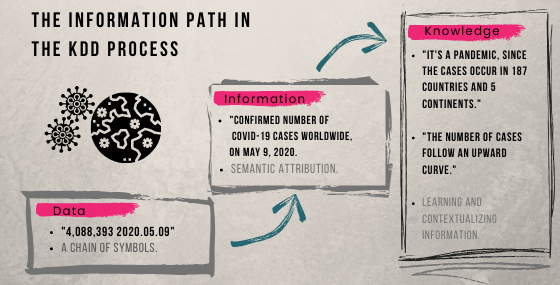

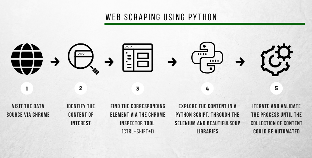
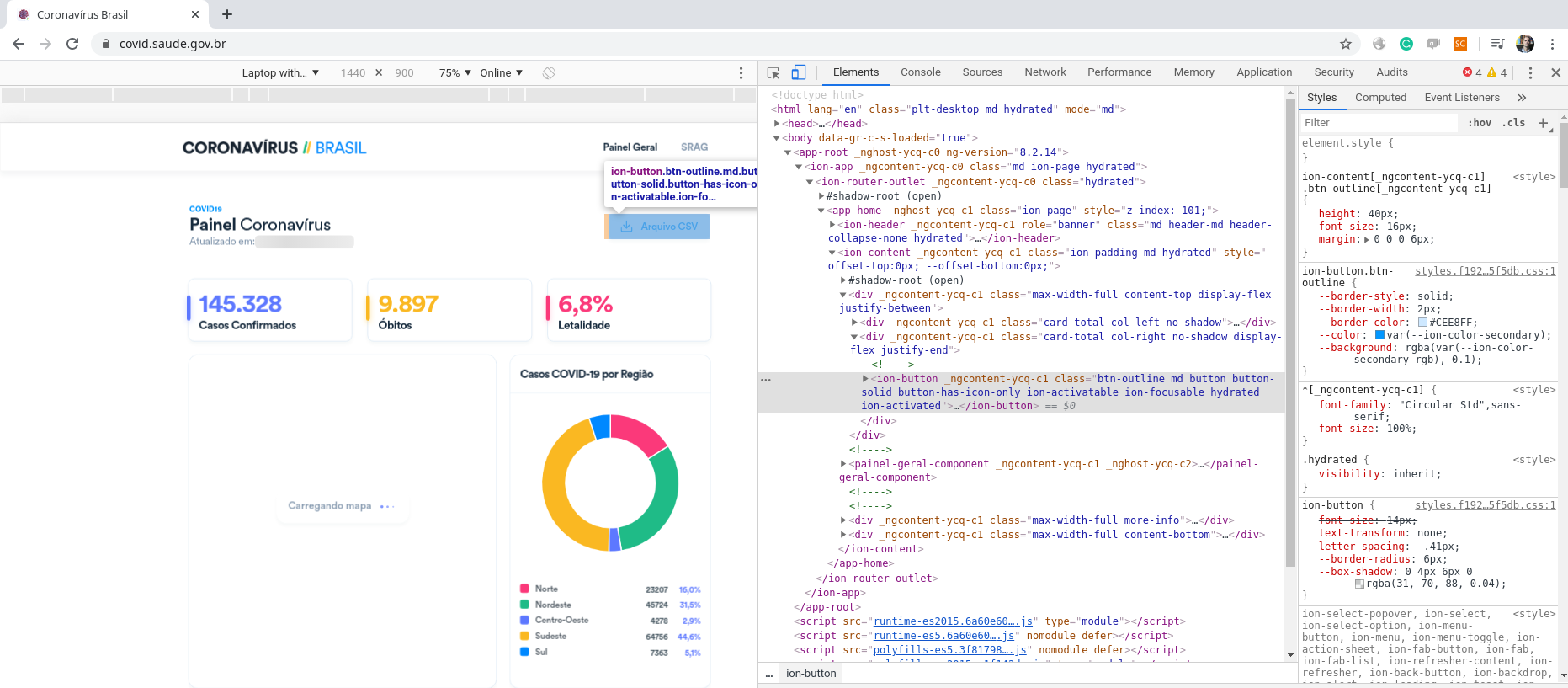

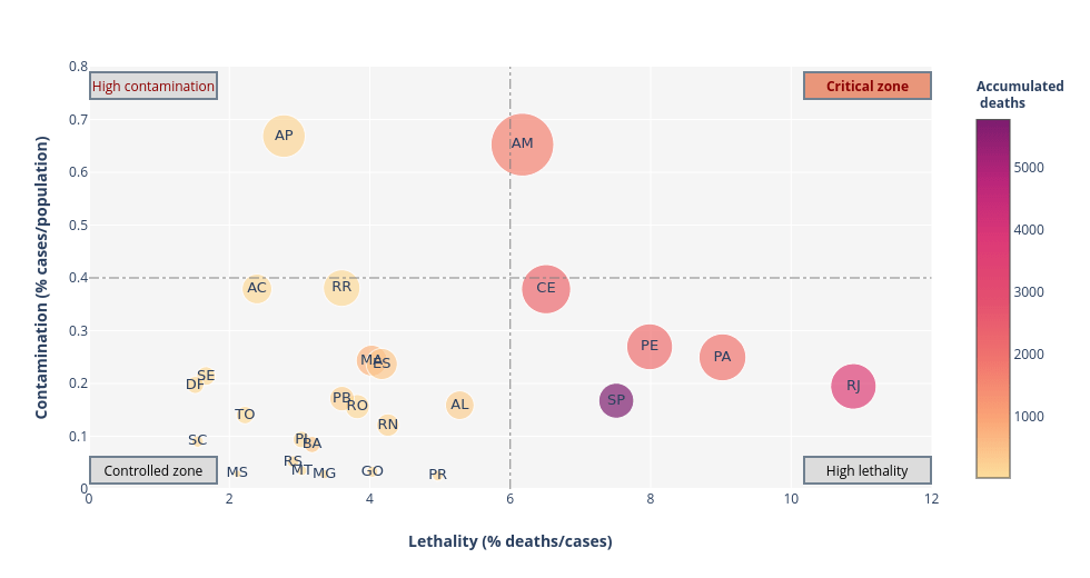

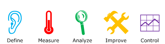

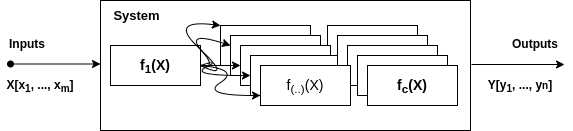
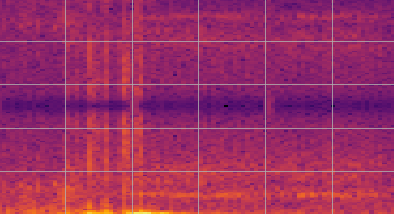


 ,
, 

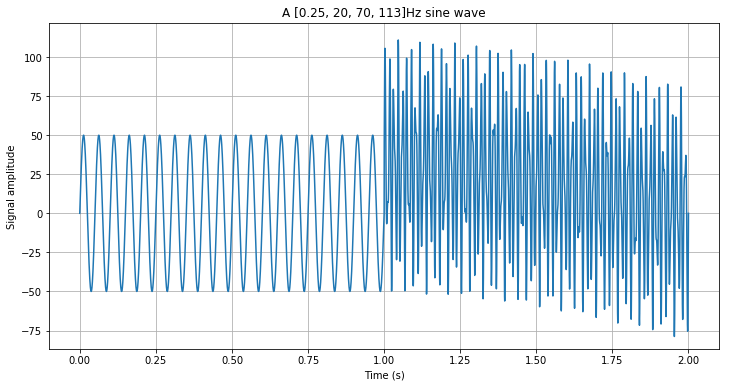
 .
. ,
, are the Fourier coefficients obtained by the Fourier transform of the signal; and
  is the harmonic base function that represents the frequency
  .
. ):
): ,
,  .
.


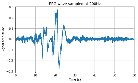
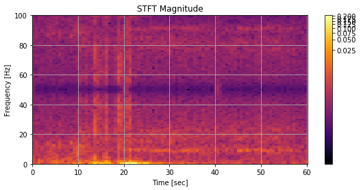


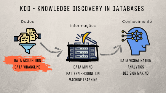
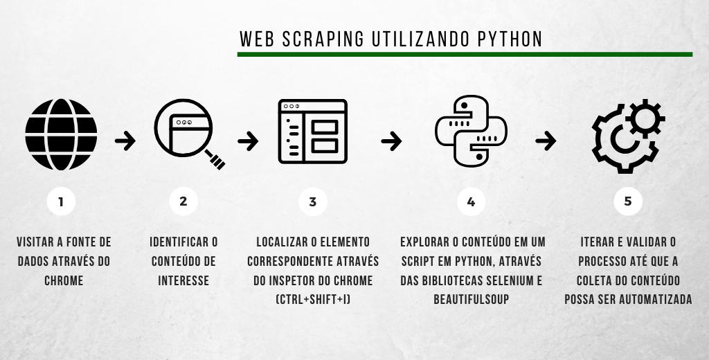


Você precisa fazer login para comentar.